Table of Contents
In 1996, the Sharpe ratio was created by William Sharpe. Since then, it’s been used as the referenced risk in finance. It is popular because of its ease of use. In 1990, Professor Sharpe was awarded a Nobel Prize in Economic Science for his effort toward CAPM. And this later contributes to its credibility.
The Sharpe Ratio was invented to provide investors with a tool to assess the performance of an investment relative to its risk. Before its introduction, investment returns were typically evaluated without adequately considering the risk involved. This ratio, developed by Nobel laureate William F. Sharpe, allows for a more comprehensive understanding by comparing the excess return of an investment to its standard deviation, a measure of risk. As a result, it offers a standardized way to determine how much additional return an investor receives for the extra volatility endured by holding a riskier asset.

What is the Sharpe ratio?
The Sharpe ratio (Sharpe index or the Sharpe measure or reward-to-variability ratio) represents a measure used to evaluate the performance of an investment by adjusting for its risk. It calculates the excess return of the investment over the risk-free rate, divided by the investment’s standard deviation, effectively quantifying return per unit of risk.


- Origin:
- It was developed by Nobel laureate economist William F. Sharpe in 1966.
- They are intended to provide a more comprehensive risk-to-reward assessment.
- Purpose:
- To measure the performance of an investment relative to its risk.
- It helps investors understand the return on an investment compared to its risk.
- Calculation:
- Formula:
.
- The risk-free rate is often represented by the yield on government securities, like U.S. Treasury bonds.
- Standard deviation measures the investment’s volatility.
- Formula:
- Interpretation:
- A higher Sharpe Ratio indicates a more favorable risk-adjusted return.
- Generally, a ratio above one is considered good, above two is very good, and above 3 is excellent.
- A negative Sharpe Ratio indicates that a risk-less asset would perform better.
- Applications:
- Financial analysts and portfolio managers widely use them.
- Useful for comparing the risk-adjusted performance of different funds or securities.
- They are often used in mutual funds, hedge funds, and portfolios.
- Limitations:
- Assumes that returns are normally distributed, which may not always be accurate.
- It is more effective for evaluating investments with symmetrical distributions of returns.
- It is less effective for portfolios with non-linear risks, such as options or leveraged investments.
- Sensitive to the chosen risk-free rate, which can vary over time.
- Variations:
- The Modified Sharpe Ratio adjusts for the skewness and kurtosis of returns.
- Other related metrics include the Sortino Ratio and Treynor Ratio, which also assess risk-adjusted returns but with different approaches to risk.
What is a good Sharpe ratio for a fund?
Usually, the good Sharpe ratio is above 1 for most investors. A Sharpe ratio higher than two is rated as very good, and the Sharpe ratio above 3.0 is considered excellent.
So, how do you calculate a Sharp ratio?
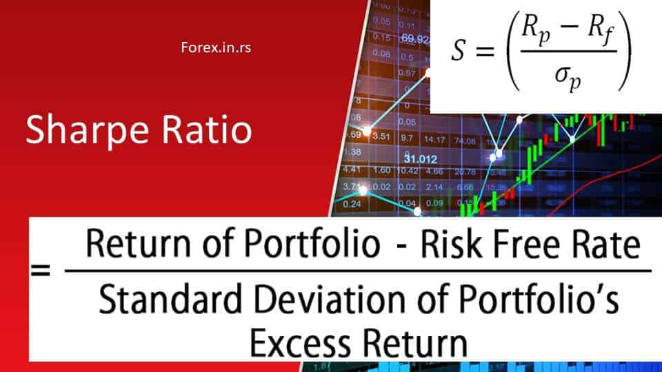
The Sharpe ratio formula is given here as:

S(x) = (Rx – Rf)/ StdDev(X)
Where;
X= the investment, Rx = x average return rate
Rf = best available rate of return, StdDev(X) = standard deviation
A. Rx, i.e., return if commonly shared, maybe per year, month, week, or day. This then reveals the shortcoming of the ratio; all returns on assets are not often customarily shared.
As we can see, the Sharpe ratio is an excellent measure of an investment’s performance. Sharpe ratio and Payoff ratio are excellent tools to analyze and compare portfolios.
A practical example of Sharp Ratio in Forex Calculation
To create a practical example of calculating the Sharpe Ratio for EUR/USD forex trading, let’s assume the following scenario:
- Time Frame: One year of trading data for the EUR/USD currency pair.
- Investment Returns: The average annual return on the investment is 8%.
- Risk-Free Rate: Assume the risk-free rate (such as the yield on a 1-year U.S. Treasury bill) is 2%.
- Standard Deviation: The standard deviation of the EUR/USD returns over the year is 5%.
Now, let’s calculate the Sharpe Ratio:
- Step 1 – Calculate Excess Return:
- Excess return = Investment Return – Risk-Free Rate
- Excess return = 8% – 2% = 6%
- Step 2 – Calculate Sharpe Ratio:
- Sharpe Ratio = Excess Return / Standard Deviation
- Sharpe Ratio = 6% / 5% = 1.2
Interpretation:
- A Sharpe Ratio of 1.2 suggests the investment has a favorable risk-adjusted return. For every unit of risk (as measured by the standard deviation), the investment yields 1.2 units of return above the risk-free rate.
- In the context of forex trading, the trading strategy for EUR/USD yields more return per unit of risk than a risk-free investment. However, when evaluating this number, traders should consider other factors, such as market conditions and risk tolerance,
How to calculate Sharp ratio video:
How to calculate Sharp ratio using Excel:
Kurtosis: This is the peakedness or flatness of a frequency distribution
Skewness graph: This is a headache to the ratio because standard deviation may not be an option when these problems occur. Sometimes, it can be risky to apply this formula when returns are not in the normal distribution.
B. The risk-free rate of return (rf): This is applied to reveal if one is appropriately rewarded for taking a further risk. Usually, the most archaic in U.S. T-bill is the risk-free rate of return. Though this kind of security is more stable, risk-free security has been debated by some that are supposed to match the period of comparable investment.
For instance, equities remain an asset that persists for an extended period. Perhaps we should not compare them with the long-term risk-free asset present: the government-issued IPS. Applying IPS that can persist for a long time would result in different ratio values because typically, under interest rate clime, T-bills have lesser returns than IPS.
For example, a decade index returned to three percent of the year 2017 on inflation-protected securities was reported by BARCLAYS US TREASURY.
In contrast, the same time, a 7.4% index return was reported by the S&P 500. One may debate that investors favoring equities over bonds were fairly rewarded. If the Sharpe ratio has a bond index of 1.16% against a 0.38% equity index, equities assets are riskier.
How to use the Sharpe ratio?
In the video below, we will see the portfolio Sharpe ratio explanation:
Sharpe ratio may be used to measure return and adjust risk to compare the investment manager’s performance.
For instance, say one investment manager makes fifteen percent returns and the other twelve percent returns. The latter looks excellent in performance. Though the latter took higher risks than the former, the former risk-adjusted return may be better. To bolster this example, a 5% free-risk rate is available; the first managers have an eight percent standard deviation, five percent for the second manager. The first would realize the Sharpe ratio of 1.25. then 1.4 goes to the second manager; this is better than the first manager. Hence, the second manager, depending on the risk-adjusted, got better returns as a result of this calculation.
NOTE:
Ratio 1: Good
Ratio2: Very good
Ratio3: Excellent
What does a negative Sharpe ratio mean
A negative Sharpe ratio means that a manager or portfolio’s performance is below the risk-free rate and can endure for long periods. Interestingly, the negative Sharpe ratio is problematic to evaluate during the volatile market. A portfolio with a slight negative excess return can be punished if its volatility is significant.
So, is a negative Sharpe ratio bad? A negative Sharpe ratio is a bad characteristic for a portfolio because it shows that it has underperformed its benchmark.
What is the Sharpe ratio of the S&P 500?
In the 21st. In the last 20 years, the average annual Sharpe ratio for the S&P 500 has been 1.2, with frequent periods of much higher and lower levels.
Bottom line
As a trader, the Sharpe Ratio is a crucial tool in my investment decision-making process. Its importance is primarily because it provides a standardized way to evaluate the risk-adjusted return of different investments. This is particularly useful in a trading environment where I often compare a diverse set of investment opportunities with varying levels of risk and return.
The Sharpe Ratio lets me understand how much excess return I am earning for the additional risk taken over a risk-free investment. This is important because not all high-return investments are desirable if they come with disproportionately high levels of risk. Using the Sharpe Ratio, I can objectively measure how much additional return I am getting for each unit of risk, which helps make more informed investment choices.
Furthermore, the Sharpe Ratio is a critical performance metric in a dynamic market environment. It helps me assess whether my trading strategy is genuinely effective or if the returns result from excessive risk-taking. A consistent metric for risk-adjusted performance is invaluable, especially in forex or stock trading, where market conditions can change rapidly.
Additionally, the Sharpe Ratio is crucial for portfolio optimization. When constructing or rebalancing my portfolio, I use the Sharpe Ratio to ensure that the overall risk-reward profile aligns with my investment objectives and risk tolerance. It aids in identifying assets that might improve the portfolio’s overall risk-adjusted returns, guiding me to allocate capital more efficiently.
Risk and compensation are evaluated together while making investment decisions, and this is the main focus of Modern Portfolio Theory.
Generally, variance or its square root drifts compensation away from the investor. So, when choosing an investment, it is advisable to deal with risk and reward together. Sharpe ratio will help make investment decisions that yield more significant returns even when the risk is considered.

He is an expert in financial niche, long-term trading, and weekly technical levels.
The primary field of Igor's research is the application of machine learning in algorithmic trading.
Education: Computer Engineering and Ph.D. in machine learning.
Igor regularly publishes trading-related videos on the Fxigor Youtube channel.
To contact Igor write on:
igor@forex.in.rs